This lesson aims at showing how to perform molecular dynamics with ABINIT using a parallel computer.
You will learn how to launch molecular dynamics calculation and what are the main input variables that govern convergence and numerical efficiency.You are supposed to know already some basics of parallelism in ABINIT, explained in the tutorial A first introduction to ABINIT in parallel, and ground state with plane waves.
This lesson should take about 1.5 hour to be done and requires to have at least a 200 CPU core parallel computer.
The basic idea underlying Ab Initio Molecular Dynamics (AIMD) is to compute the forces acting on the nuclei from electronic structure calculations that are performed as the molecular dynamics trajectory is generated. An AIMD calculation assumes only that the system is composed of nuclei and electrons, that the Born–Oppenheimer approximation is valid, and that the dynamics of the nuclei can be treated classically on the ground-state electronic surface. It allows both equilibrium thermodynamic and dynamical properties of a system at finite temperature to be computed. For example melting temperatures, phase transitions, atomic vibrations, structure factor... but also XANES or IR spectrum can be obtained with this technique. AIMD deals with supercells of hundred to thousand of atoms (usually, the larger, the better!). In addition Molecular Dynamics simulations can be performed for days, weeks or even months! They are therefore very time consuming and can not be done without the help of high speed and massively parallel computing.
Before continuing, you might
consider to work in a different
subdirectory as for the other lessons. Why not "Work_paral_moldyn" ?
In what follows, the name of files are
mentioned as if
you were in this subdirectory.
All the input files can be found in the ~abinit/tests/tutorial/Input
directory.
In the following, when "run ABINIT over nn CPU cores" appears, you have to use a specific command line according to the operating system and architecture of the computer you are using. This can be for instance: mpirun -n nn abinit < abinit.files or the use of a specific submission file.
You can compare your results with several reference
output files located in ~abinit/tests/tutorial/Refs
and ~abinit/tests/tutorial/Refs/
There are different algorithms to do molecular dynamics.
See the input variable "ionmov",
with values 1, 6, 7, 8, 9, 12, 13 and 14.
The input file tmoldyn_01.in
is an example of a file
that contains data for a molecular dynamics simulation using the isokinetic ensemble for aluminum.
Open the tmoldyn_01.in
file and look at it carefully. The
unit cell is defined at the end. It is a 2x2x2 fcc supercell containing 32 atoms of Al. ionmov is set to 12 for the isokinetic ensemble, and since ntime is set to 50, ABINIT
will carry on 50 time steps of molecular dynamics. The calculation will
be performed for a temperature of 3000 K, see the key variable mdtemp. It
gives the initial and final temperature in Kelvin of the
simulation. The temperature will change linearly from the initial
temperature
mdtemp(1) at itime=1 to
the final temperature mdtemp(2) at the end of the
ntime timesteps.
Here the temperature will stay constant during the whole simulation.
Note that we use the same temperature for the ions and the electrons : occopt has been set to 3 for a Fermi-Dirac smearing and tsmearr
has been set to 3000 Kelvin. Nothing prevent you to use different
electronic and ionic temperature, you just have to know why you are
doing so!
Molecular dynamics simulations are always large calculations, dealing with supercells of hundreds to thousands of atoms. Therefore they are always performed in parallel. In tmoldyn_01.in, paral_kgb has been set to 1 to activate the parallelisation over K-points, G-vectors and bands. The three following keywords give the number of processors for each level of parallelisation. Since we have only one K-point in the simulation (the gamma point), nkpt has been set to 1. npfft is set to 3 and npband to 10, for a total number of 3x10=30 processors. You might use the tmoldyn.files file. Edit it and adapt it with the appropriate file names.
Then run the calculation in parallel over 30 CPU cores. You can change the distribution of processors over the level of parallelisation to try to find the most efficient one. Set for example npfft to 1 and npband to 40. You can make other choices and compare the individual cpu time. Since molecular dynamics can last for weeks, it is crucial to find the appropriate distribution to reduce the computational time at the maximum. Look at the output file. For each iteration you will see the coordinates, the forces, the velocities and the kinetic and the total energy.
In addition, ABINIT should have generated a HIST file, which contains the whole history of the molecular dynamics simulation : atomic positions, velocities, primitive translations, stress tensor, energies... at each time step. This file will be used to restart the calculation if you want to perform more time steps or to extract the necessary informations to make use of the molecular dynamics simulation. In tmoldyn_01.in add the keyword restartxf and set it to -1. Run the calculation again, in the same directory. Look at the new output file. The number of each time step are indicated over the total number of steps :
--- Iteration: ( 1/100) Internal Cycle: (1/1)
Since we already performed 50 steps of molecular dynamics, the total number of time steps are now 100. So the first 50 iterations are from the previous calculation. You can check that by comparing tmoldyn_01.out and tmoldyn_01.outA. There is only one HIST file and it contains the history of the two calculations.
Now we can calculate and plot several quantities. We need
for that the diag_moldyn.py python script. You can find it in the ~abinit/doc/tutorial/lesson_paral_moldyn directory (link here).
Run the diag_modyn.py script (type: "python diag_moldyn.py").
You can read (on standard output) the average value and the standard deviation of the total energy, the temperature and the pressure. You have also generated several files which contain pressures, energies, stresses, positions and temperatures. You can plot this files to observe the behavior of the quantities during the molecular dynamics. Note that 100 time steps is far from being sufficient to equilibrate physical quantities as pressure. 2000 or 3000 are more common numbers to reach this goal but it would exceed the time alloted to this tutorial.
1.a Computing the convergence in K-points
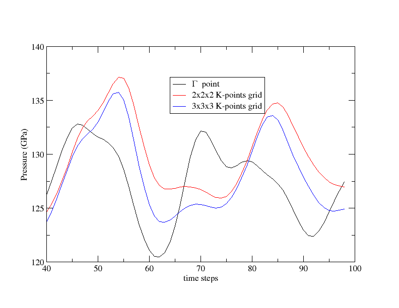
The files tmoldyn_02.in and tmoldyn_03.in are input files for 2x2x2 and 3x3x3 K-points grid respectively, or 4 and 14 K-points in the irreducible Brillouin zone. Since the parallelisation is the most efficient over the k-point level you should always put nkpt to the largest possible value before increasing npfft and npband. We have followed this rule in the input files. Change the name of the previous file PRESS to PRESS01 to save it. Run now ABINIT in parallel over 120 CPU cores with tmoldyn_02.in and over 140 CPU cores with tmoldyn_03.in. At the end of each calculation use the diag_moldyn.py script and save the results in PRESS02 and PRESS03. You can now plot the pressures in term of the K-points grids and compare the average values:
As said previously our simulations are too short to be completely convincing but you can see that you need at least a 2x2x2 K-points grid for a 32 atoms cell. If you have some time, increase ntime to 300 and run again ABINIT.
1.b Computing the convergence in cell size
We also have to check if our cell is sufficiently large to give reliable physical quantities. In the previous section we used a 2x2x2 fcc supercell. tmoldyn_04.in is an input file for a 3x3x3 fcc supercell and therefore contains 108 atoms. nband and acell has been scaled accordingly to take into account the new size of the cell. Run now ABINIT in parallel over 45 CPU cores and then diag_moldyn.py (note that the output file is very big, and no reference has been provided for comparison). Save the pressure to PRESS04. tmoldyn_05.in has the same cell but a 2x2x2 K-points grid (note that the output file is very big, and no reference has been provided for comparison). Run it over the adequate number of cores and save the pressure to PRESS05. Plot now PRESS04 and PRESS05 and compare the average values. You'll see that for this size of cell, the gamma point is sufficient.
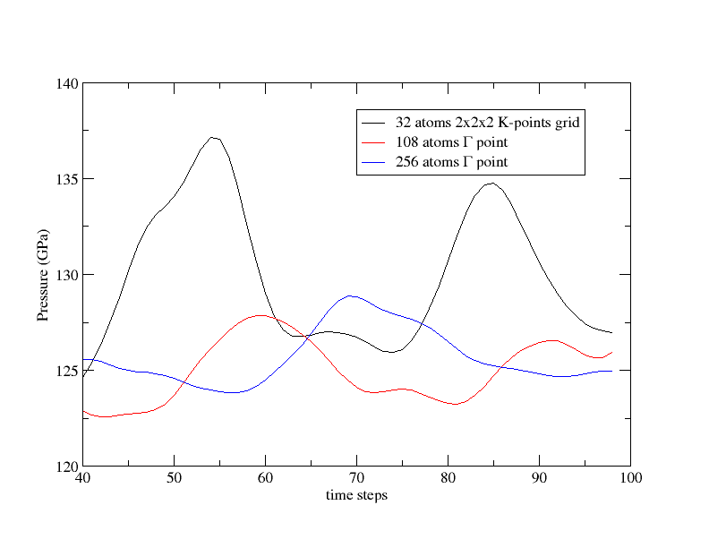
We are now going to increase again the cell size. With a 4x4x4 fcc cell, the file tmoldyn_06.in has 256 atoms. Of course, nband and acell has been scaled. This calculation should last for 30 min over 60 CPU cores (note that the output file is very big, and no reference has been provided for comparison). Run it and save the pressure to PRESS06. Plot now PRESS02, PRESS04 and PRESS06, remove the first steps and compare the pressure average values: