This lesson aims at showing how to get the following physical properties, for periodic solids:
For the theory related to the temperature-dependent calculations, you can read the following papers: [Ponce2015], [Ponce2014] and [Ponce2014a].
There are two ways to compute the temperature dependence with Abinit:
This lesson should take about 1 hour to be done.
The reference input files for this lesson are located in ~abinit/tests/tutorespfn/Input and the corresponding reference output files are in ~abinit/tests/tutorespfn/Refs. The prefix is "tdepes". First, run the calculation using the ~abinit/tests/tutorespfn/Input/tdepes_1.in input file. You can use the files file ~abinit/tests/tutorespfn/Input/tdepes_1.files for abinit (will always be the same, just change the last digit for the other calculations):
python temperature_para.pyand enter the informations that the script ask. For example a possibility could be (please remove the comments if you plan to use this file as input for the script):
1                     # Number of cpu to do the calculations
1                     # Static ZPR computed in the Allen-Heine-Cardona (AHC) theory
temperature           # Root name of the output
y                     # We want the ZPR AND the temperature dependence
1000 50               # We want the renormalization between 0 and 1000K by steps of 50K.
y
1                     # Number of Q-points we have (here we only computed $\Gamma$)
tdepes_1o_DS3_DDB       # Name of the response-funtion (RF) DDB file
tdepes_1o_DS2_EIG.nc    # Eigenvalues at $\mathbf{k+q}$
tdepes_1o_DS3_EIGR2D.nc # Second-order electron-phonon matrix element
tdepes_1o_DS3_EIGI2D.nc # Second-order electron-phonon matrix element for electronic lifetime
tdepes_1o_DS1_EIG.nc    # Eigenvalues at $k$
The python code will generate 3 files:
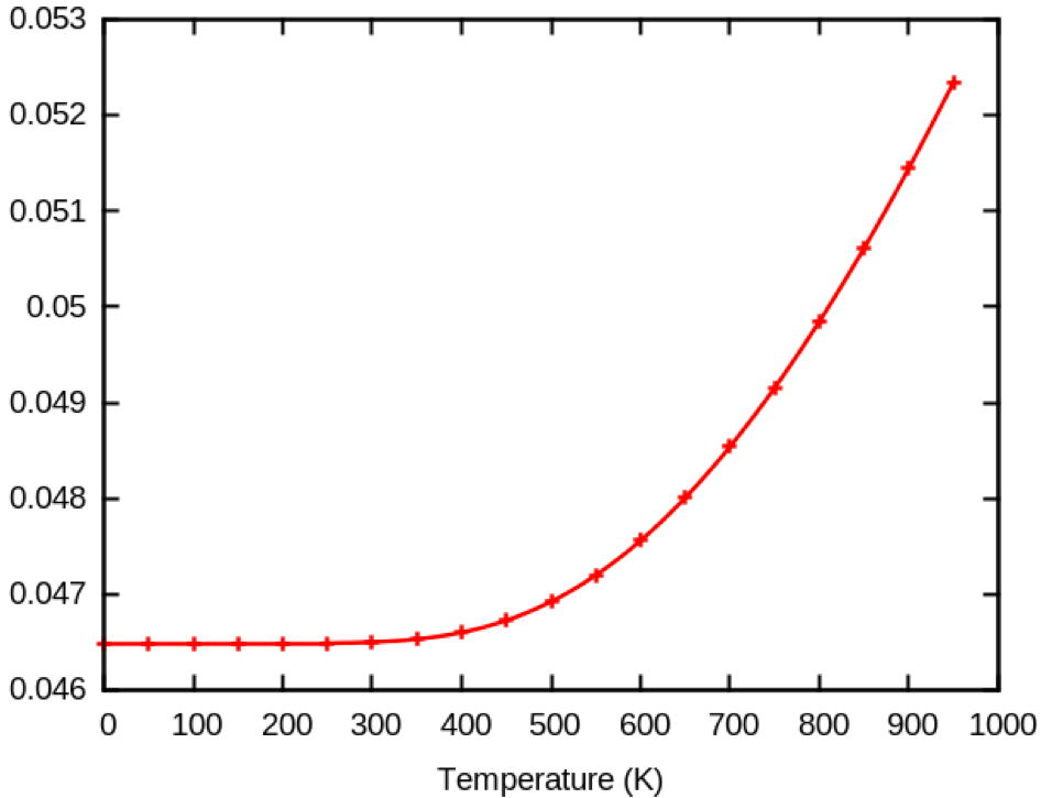
Here you can see that the HOMO correction goes down with temperature.
This is due to the underconvergence of the calculation.
If you increase ecut from 5 to 10, you get the following plot.
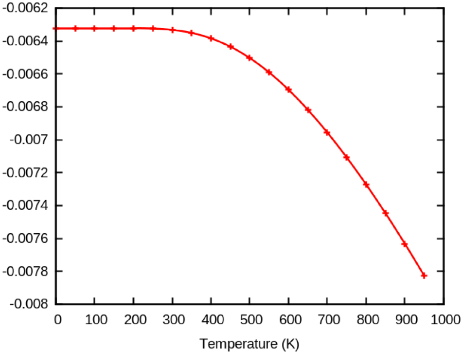
Now, the HOMO eigenenergies correction goes up with temperature... You can also plot the LUMO eigenenergies corrections and see that they go down. The ZPR correction as well as their temperature dependence usually closes the gap in semiconductors.
From now on we will only describe the approach with Abinit compiled with Netcdf. The approach with Anaddb is similar to what we described above. Note that Anaddb only support homogenous q-point grid integration. You can integrate over the q-grid using either random q-point integration or homogenous Monkhorst-Pack based integration. For the random integration you should create a script that generate random q-point, perform the Abinit calculations at these points and then integrate them using the temperature_para.py script. The script will detect that you did random integration thanks to the weight of the q-point stored in the _EIGR2D.nc file and perform the integration accordingly. The random integration converges slowly but in a consistent manner. Since this methods is a little bit less user friendly we will focus on the homogenous integration. The first thing we need to do is to determine the number of q-point in the IBZ for a given q-point grid. We choose here a 4x4x4 q -point grid. Use the input file ~abinit/tests/tutorespfn/Input/tdepes_3.in. Launch this job, and kill it after a few seconds. Then look into the log file to find the following line after the list of q-points:
symkpt : the number of k-points, thanks to the symmetries,
is reduced to     8
In general, in order to get the number of q-points, launch a "fake" run with a k-point grid equivalent to the q-point grid you want to use in your calculation. Now that we know that the 4x4x4 q-point grid reduces to 8 IBZ q-point we can make the following substitution into the input file
ndtset 3 udtset 1 3 ==> ndtset 24 udtset 8 3and then launch the calculation. When the Abinit run is finished, launch the python script
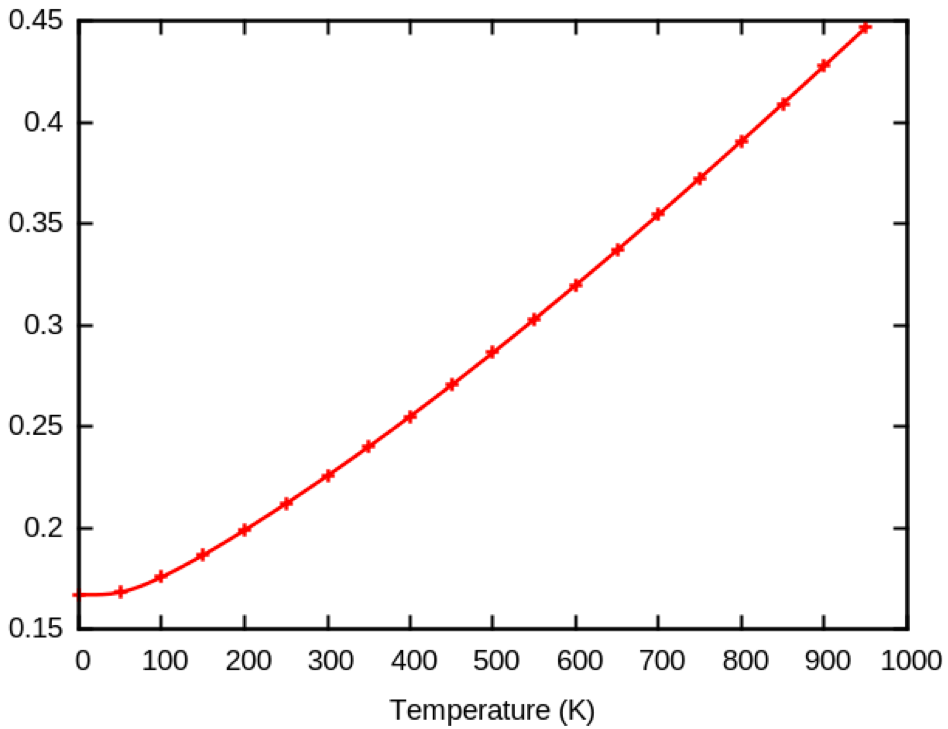
python temperature_para.py < tdepes_3.fileswith the file ~abinit/tests/tutorespfn/Input/tdepes_3.files. The plotting of the same HOMO band at k=Γ for a 4x4x4 q-point grid gives a very different result than previously (this graph has been obtained with ecut = 10).
As a matter of fact, diamond needs an extremely dense q-point grid (40x40x40) to be converged.
On the bright side each q-point calculation is independent and thus the parallel scaling is ideal...
Go to the top
The calculation of the electronic eigenvalue correction due to electron-phonon coupling along high-symmetry lines requires the use of 6 datasets per q-point. Different datasets are required to compute the following quantites:
Run the calculation using the ~abinit/tests/tutorespfn/Input/tdepes_4.in input file, then the files file ~abinit/tests/tutorespfn/Input/tdepes_4.files for the python script. Of course, the high symmetry points that we computed in section 2 have the same value here. It is a good idea to check it by running the script with the file ~abinit/tests/tutorespfn/Input/tdepes_3bis.files.
You can then copy the plotting script (Plot-EP-BS) python file from ~abinit/scripts/post_processing/plot_bs.py
into the directory where you did the Abinit calculations.
Note that in order to run this script you need:
tdepes_4_EP.nc
L \Gamma X W K L W X K \Gamma
-20 30
0
This should give you the bandstructure
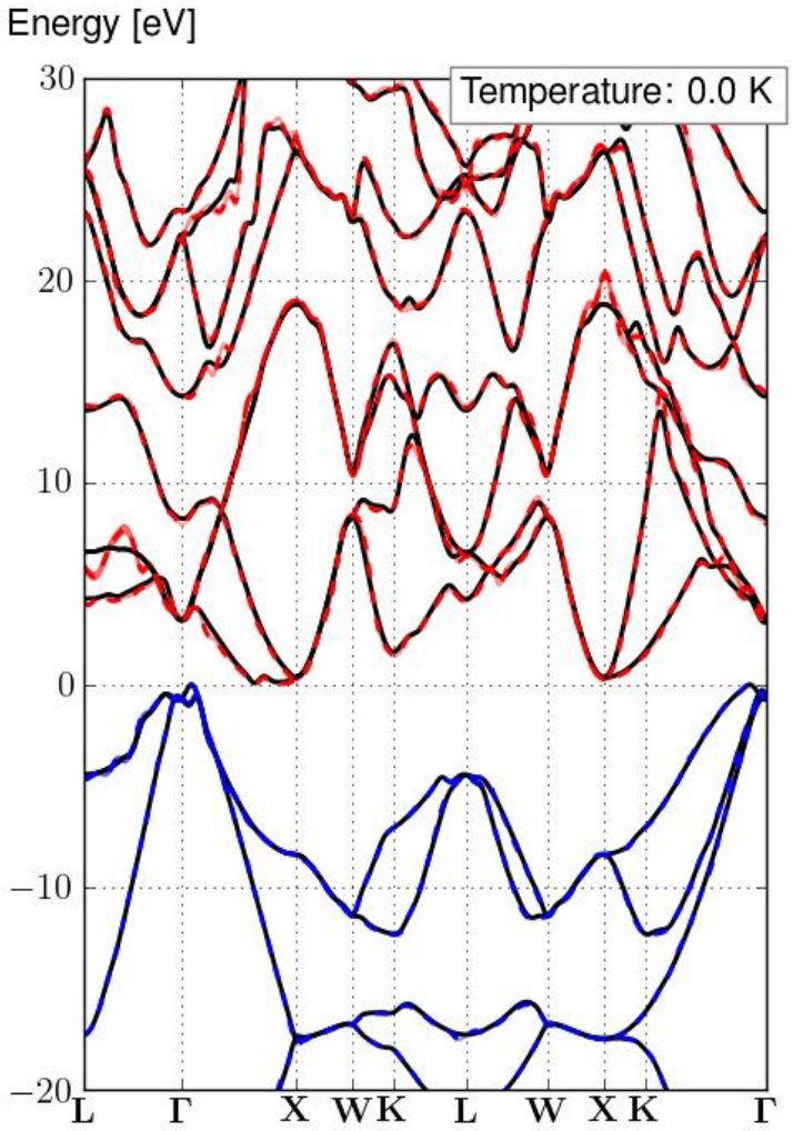
where the solid black lines are the traditional electronic bandstructure, the dashed lines are the electronic eigenenergies with electron-phonon renormalization at a defined temperature (here 0K). Finally the area around the dashed line is the lifetime of the electronic eigenstates.
You should of course notice all the spiky jumps in the renormalization. This is because we did a completely under-converged calculation.
It is possible to converge the calculations using ecut=30 Ha, a ngkpt grid of 6x6x6 and an increasing ngqpt grid to get converged results:
| Convergence study ZPR and inverse lifetime(1/τ) [meV] at 0K               |
| q-grid   | Nb qpt |       Γ25'       |        Γ15       |      Min Γ-X     |
|          | in IBZ |  ZPR   |  1/τ   |   ZPR   |  1/τ   |   ZPR   |  1/τ   |
| 4x4x4    |  8     | 0.1175 | 0.0701 | -0.3178 | 0.1916 | -0.1570 | 0.0250 |
| 10x10x10 |  47    | 0.1390 | 0.0580 | -0.3288 | 0.1847 | -0.1605 | 0.0308 |
| 20x20x20 |  256   | 0.1446 | 0.0574 | -0.2691 | 0.1823 | -0.1592 | 0.0298 |
| 26x26x26 |  511   | 0.1448 | 0.0573 | -0.2736 | 0.1823 | -0.1592 | 0.0297 |
| 34x34x34 |  1059  | 0.1446 | 0.0573 | -0.2699 | 0.1821 | -0.1591 | 0.0297 |
| 43x43x43 |  2024  | 0.1447 | 0.0572 | -0.2650 | 0.1821 | -0.1592 | 0.0297 |
As you can see the limiting factor for the convergence study is the convergence of the LUMO band at Γ. This band is not the lowest in energy (the lowest is on the line between Γ and X) and therefore this band is rather unstable. This can also be seen by the fact that it has a large electronic broadening, meaning that this state will decay quickly into another state.
Using the relatively dense q-grid of 43x43x43 we can obtain the following converged bandstructure, at a high temperature (1900K):
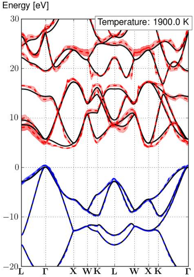
Here we show the renormalization at a very high temperature of 1900K in order to highlight more the broadening and renormalization that occurs. If you want accurate values of the ZPR at 0K you can look at the table above.