ABINIT tutorial : parallelism in the linear-response case.
This lesson aims at showing how to use the parallelism for all the properties that are computed
on the basis of the linear-response part of ABINIT, i.e. :
- responses to atomic displacements (to compute phonon frequencies, band structures, ... )
- responses to homogeneous electric fields (dielectric constant, Born effective charges, Infra-red characteristics )
- responses to strain (elastic constants, piezoelectric constants ...)
Such computations are realized when one of the input variables
rfphon,
rfelfd or
rfstrs
are non-zero,
which activates optdriver=1.
You are supposed to be well-familiarized with such calculations before starting the present tutorial.
See the input variables described in the file VARRF
and the tutorial Response-Function 1 and subsequent tutorials.
You will learn about the basic implementation of parallelism for linear-response calculations,
then will execute a very simple, quick calculation for one dynamical matrix for FCC aluminum, whose
scaling is limited to a few dozen computing cores, then you will execute
a calculation whose scaling is much better, but that would take
a few hours in sequential, using a provided input file.
For the last section of that part, you would be better off having access to more than 100 computing cores, although
you might also change the input parameters to adjust to the machine you have at hand.
For the other parts of the tutorial, a 16-computing-core machine is recommended,
in order to perform the scalability measurements.
This lesson should take less than two hours to be done if a powerful parallel computer is available.
You are supposed to know already some basics of parallelism in ABINIT, explained in the tutorial
A first introduction to ABINIT in parallel.
Copyright (C) 2000-2014 ABINIT group (XG,RC)
This file is distributed under the terms of the GNU General Public License, see
~abinit/COPYING or
http://www.gnu.org/copyleft/gpl.txt .
For the initials of contributors, see ~abinit/doc/developers/contributors.txt .
Contents of lesson paral_dfpt:
- 1. The structure of the parallelism for the linear-response (Density-Functional Perturbation Theory) part of ABINIT
- 2. Computation of one dynamical matrix (q =0.25 -0.125 0.125) for FCC aluminum
- 3. Computation of one perturbation for a slab of 29 atoms of barium titanate
1.1. Let us recall first the basic structure of typical linear-response calculations. This is summarized in box 1.
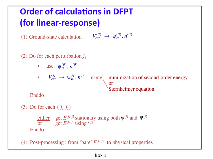
The step 1 is done in a preliminary ground-state calculation (either by an independent run,
or by computing them using an earlier dataset before the linear-response calculation).
The parallelisation of this step is examined in a separate lesson.
The step 2 and step 3 are the time-consuming linear-response steps, to which the present tutorial is dedicated,
and for which the implementation of the parallelism will be explained. They generate different files, and in particular,
one (or several) DDB file(s). As explained in related tutorials (see e.g. Response-Function 1),
several perturbations are usually treated in one dataset (hence the "Do for each perturbation"-loop in step 2 of this Schema). For example,
in one dataset, although one considers only one phonon wavevector, all the primitive atomic displacements for this wavevector
(as determined by the symmetries) can be treated in turn.
The step 4 refers to MRGDDB and ANADDB post-processing of the DDB generated by steps 2 and 3. These are not time-consuming
sections. No parallelism is needed.
1.2. The equations to be considered for the computation of the first-order wavefunctions and potentials (step 2 of box 1),
which is the really time-consuming part of any linear-response calculation, are presented in box 2.
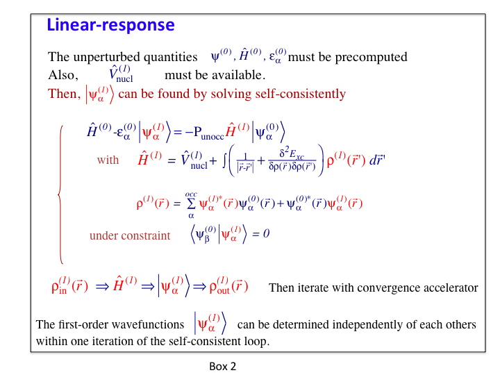
The parallelism currently implemented for the linear-response part of ABINIT is based on
the parallel distribution of the most important arrays: the set of first-order and ground-state wavefunctions.
While each such wavefunction is stored completely in the memory linked to one computing core (there is no splitting
of different parts of one wavefunction between different computing cores - neither in real space nor in reciprocal space),
different such wavefunctions might be distributed over different computing cores.
This easily achieves a combined k point, spin and band index parallelism, as explained in box 3.
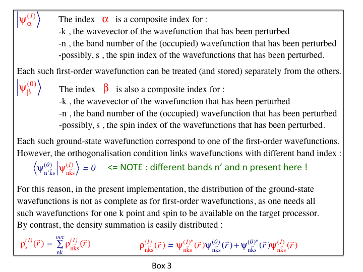
1.3. The parallelism over k points, band index and spin for the set of wavefunctions is implemented in all relevant steps,
except for the reading (initialisation) of the ground-state wavefunctions (from an external file). Thus, the most CPU time-consuming
parts of the linear-response computations are parallelized.
The following are not parallelized :
- input of the set of ground-state wavefunctions
- computing the first-order change of potential from the first-order density,
and similar operations that do not depend on the bands or k points.
In the case of small systems, the maximum achievable speed-up will be limited by the input of the set of ground-state wavefunctions.
For medium to large systems, the maximum achievable speed-up will be determined by the operations that do not depend
on the k point and band indices.
Finally, the distribution of the set of ground-state wavefunctions to the computing cores
that need them is partly parallelized, as no parallelism over bands can be exploited.
Before continuing you might work in a different subdirectory as
for the other lessons. Why not "work_paral_dfpt" ?
All the input files can
be found in the ~abinit/tests/tutoparal/Input directory.
You might have to adapt them to the path of the directory in which you have decided to perform your runs.
You can compare your
results with reference output files located in
~abinit/tests/tutoparal/Refs.
In the following, when "(mpirun ...) abinit" appears, you have
to use a specific command line according to the operating system and
architecture of the computer you are using. This can be for instance:
mpirun -np 16 abinit
We start by treating the case of a small systems, namely FCC aluminum, for which there is only one atom
per unit cell. Of course, many k points are needed.
The input files can be found in the directory ~abinit/tests/tutoparal/Input .
2.1. The first step is the precomputation of the ground state wavefunctions.
This is driven by the files tdfpt_01.files (and tdfpt_01.in).
You should edit them and examine them.
One relies on a k-point grid of 8x8x8 x 4 shifts (=2048 k points), and 5 bands.
For this ground-state calculation, symmetries can be used to reduce drastically the number of k points :
there are 60 k points in the irreducible Brillouin zone (this cannot be deduced from the examination of the
input file, though). This calculation is very fast, actually.
You can launch it :
(mpirun ...) abinit < tdfpt_01.files > tdfpt_01.log
A reference output file is available in ~abinit/tests/tutoparal/Refs , under the name tdfpt_01.out .
It was obtained using 4 computing cores, and took a few seconds.
2.2. The second step is the linear-response calculation, for which the files are
tdfpt_02.files (and tdfpt_02.in).
There are three perturbations (three atomic displacements). For the two first perturbations, no symmetry can be used,
while for the third, two symmetries can be used to reduce the number of k points to 1024.
Hence, for the perfectly scalable sections of the code, the maximum speed up is 5120 (=1024 k points * 5 bands),
if you have access to 5120 computing cores.
However, the sequential parts of the code dominate at a much, much lower value.
Indeed, the sequential parts is actually a few percents of the
code on one processor, depending on the machine you run. The speed-up might saturate beyond 4 and 8 (depending on the machine).
First copy the output of the ground-state calculation so that it can be used as the input of the
linear-response calculation :
cp tdfpt_01.o_WFK tdfpt_02.i_WFK
cp tdfpt_01.o_WFK tdfpt_02.i_WFQ
Then, you can launch the calculation :
(mpirun ...) abinit < tdfpt_02.files > tdfpt_02.log
A reference output file is given in ~tests/tutoparal/Refs , under the name tdfpt_02.out .
Edit it, and examine some information ...
The calculation has been made with four computing cores :
- nproc = 4
The wall clock time is less than 50 seconds :
-
- Proc.   0 individual time (sec): cpu=         48.5  wall=         48.5

================================================================================

 Calculation completed.
.Delivered    0 WARNINGs and   3 COMMENTs to log file.
+Overall time at end (sec) : cpu=        194.1  wall=        194.1
The major result is the phonon frequencies :
  Phonon wavevector (reduced coordinates) :  0.25000 -0.12500  0.12500
 Phonon energies in Hartree :
   6.944980E-04  7.756637E-04  1.145943E-03
 Phonon energies in meV     :
-  1.889825E+01  2.110688E+01  3.118270E+01
 Phonon frequencies in cm-1    :
-  1.524247E+02  1.702385E+02  2.515054E+02
 Phonon frequencies in Thz     :
-  4.569578E+00  5.103622E+00  7.539943E+00
 Phonon energies in Kelvin  :
-  2.193049E+02  2.449349E+02  3.618597E+02
2.3. Because this test case is quite fast, you should play a bit with it. In particular,
run it several times, with an increasing number of computing cores (let's say, up to 32 computing cores, at which stage you should have obtained
a saturation of the speed-up).
You should be able to obtain the following.
- The result is independent (to an exquisite accuracy) of the number of computing cores that is used
- The timing section reveals that the reading of the ground-state wavefunction file is the limiting step for the parallelisation
Concerning the latter, you will need to understand, in the output file, the timing section. It is present a bit before
the end of the output file :
-
- For major independent code sections, cpu and wall times (sec),
-  as well as % of the time and number of calls for node 0-
- routine                        cpu     %       wall     %      number of calls
- fourwf(pot)                   19.834  10.2     19.794  10.2         187989
- inwffil                        7.387   3.8      7.390   3.8             10
- fourwf(G->r)                   6.721   3.5      6.869   3.5         116049
- cgwf3-O(npw)                   2.226   1.1      2.228   1.1             -1
- vtorho3-kpt loop               2.181   1.1      2.163   1.1             33
- nonlop(forces)                 1.924   1.0      1.947   1.0          90880
- projbd                         1.775   0.9      1.734   0.9         318634
- nonlop(apply)                  1.690   0.9      1.719   0.9         116309
- vtowfk3(contrib)               1.654   0.9      1.556   0.8             -1
- 61   others                    2.819   1.5      2.803   1.4
-
- subtotal                      48.211  24.8     48.203  24.8

- For major independent code sections, cpu and wall times (sec),
- as well as % of the total time and number of calls

- routine                         cpu     %       wall     %      number of calls
-                                                                  (-1=no count)
- fourwf(pot)                   79.067  40.7     79.326  40.9         752230
- inwffil                       29.548  15.2     29.560  15.2             40
- fourwf(G->r)                  25.828  13.3     25.898  13.3         447552
- cgwf3-O(npw)                   9.096   4.7      9.081   4.7             -4
- vtorho3-kpt loop               8.672   4.5      8.611   4.4            132
- nonlop(forces)                 7.707   4.0      7.716   4.0         363520
- projbd                         6.925   3.6      6.668   3.4        1275084
- nonlop(apply)                  6.810   3.5      6.864   3.5         465510
- vtowfk3(contrib)               6.280   3.2      6.199   3.2             -4
- getghc-other                   3.176   1.6      3.195   1.6             -4
- status                         2.615   1.3      2.534   1.3         919162
- vtorho3:synchro                2.029   1.0      2.040   1.1            132
- 58   others                    4.175   2.2      4.217   2.2

- subtotal                     191.928  98.9    191.909  98.9
It is made of two groups of data. The first one corresponds to the analysis of the timing
for the computing core (node) number 0 . The second one is the sum over all computing cores
of the data of the first group. Note that there is a factor of four between these two groups,
reflecting that the load balance is good.
Let's examine the second group of data in more detail. It corresponds to a decomposition
of the most time-consuming parts of the code. Note that the subtotal is 98.9 percent, thus
the statistics is quite good. Without going into the detail of each routine,
for the present purpose, the most significant information is that among all the
timed sections of the code, only "inwffil" and "vtorho3:synchro" will not benefit from
parallelism.
"inwffil" is a subroutine whose job is to read the ground-state wavefunctions
(you can find the source of the "inwffil" routine in the latest ABINIT sources).
As mentioned in the section 1, the reading of the ground-state wavefunctions is not done in parallel in the case of the linear-response
computations (note that the reading is actually parallelized for e.g. ground-state calculations).
In the output file provided as a reference (with four computing cores), the "inwffil" wall clock time
is 7.387 seconds, on a total of 48.211 secs. By increasing the number of computing cores, it will be
possible to decrease the total time, but not below the value of 7.387 seconds in any case.
You should observe a similar behaviour with your own tests.
3.1. This test, with 29 atoms, is slower, but scales better than the Al FCC case. It consists in the
computation of one perturbation at qpt 0.0 0.25 0.0 for a 29 atom slab of barium titanate, artificially terminated
by a double TiO2 layer on each face, with a reasonable
k-point sampling of the Brillouin zone.
The symmetry of the system and perturbation will allow to decrease this sampling to one quarter of the Brillouin zone.
E.g. with the k-point sampling ngkpt 4 4 1 , there will be actually 4 k-points in the irreducible Brillouin zone for the Ground state calculations.
For the response-function case, only one symmetry will survive, so that, after the calculation of the frozen-wavefunction part
(for which no symmetry is used), the self-consistent part will be done with 8 k points in the corresponding irreducible Brillouin zone.
With the sampling 8 8 1, there will be 32 k points in the irreducible Brillouin zone for the linear-response case.
There are 120 bands.
Note that the value of ecut that is used in the present
tutorial is too low to obtain physical results (it should be around 40 Hartree).
As in the previous case, a preparatory ground-state calculation is needed.
The input files are provided, in the directory ~abinit/tests/tutoparal/Input .
The preparatory step is governed by tdfpt_03.files (and tdfpt_03.in). The
real (=linear-response) test case is governed by tdfpt_04.files (and tdfpt_04.in).
The reference output files are present in ~abinit/tests/tutoparal/Refs :
tdfpt_0324.out and tdfpt_0432.out . The naming convention is such that the number of cores
used to run them is added after the name of the test : the tdfpt_03.in file was run with 24 cores,
while the tdfpt_04.in was run with 32 cores.
The preparatory step took about 5 minutes, and the linear-response step took about 5 minutes as well.
You can run now these test cases. For tdfpt_03, you might need to change the npband value (presently 6), if you are not
using 24 processors. At variance, for tdfpt_04, no adaptation of the input file is needed to be able to run on an arbitrary
number of processors.
To launch the ground-state computation, type :
(mpirun ...) abinit < tdfpt_03.files > tdfpt_03.log
then copy the output of the ground-state calculation so that it can be used as the input of the
linear-response calculation :
cp tdfpt_03.o_WFK tdfpt_04.i_WFK
cp tdfpt_03.o_WFK tdfpt_04.i_WFQ
and launch the calculation :
(mpirun ...) abinit < tdfpt_04.files > tdfpt_04.log
Now, examine the obtained output file for test 04, especially the timing.
In the reference file ~abinit/tests/tutoparal/Refs/tdfpt_0432.out , with 32 computing cores,
the timing section delivers :
- For major independent code sections, cpu and wall times (sec),
- as well as % of the total time and number of calls

- routine                         cpu     %       wall     %      number of calls
-                                                                  (-1=no count)
- projbd                      3046.599  34.0   3065.259  34.0         171639
- fourwf%(pot)                2545.342  28.4   2561.313  28.4         103098
- nonlop(apply)               1059.279  11.8   1066.034  11.8          85818
- fourwf%(G->r)                531.322   5.9    534.929   5.9          50112
- vtorho3:synchro              444.450   5.0    448.598   5.0            576
- nonlop(forces)               195.017   2.2    195.487   2.2         100800
- newkpt(excl. rwwf   )        179.142   2.0    179.185   2.0            -32
- vtowfk3(contrib)             137.486   1.5    137.878   1.5            -32
- pspini                        97.276   1.1     99.901   1.1             32

<...>

- 45   others                    0.000   0.0      0.000   0.0

- subtotal                    8760.405  97.8   8811.874  97.8
You will notice that the sum of the major independent code sections is again very close to 100%.
You might now explore the behaviour of the CPU time for different numbers of compute cores
(consider values below and above 32 processors).
Some time-consuming routines will benefit from the parallelism, some other will not.
The kpoint+band parallelism will efficiently work for many important sections of the code :
projbd, fourwf%(pot), nonlop(apply), fourwf%(G->r). In this test,
the product nkpt (the effective number of k points for the current perturbation) times nband is
8*120=960. Of course, the total speed-up will saturate well below this value, as there are some
non-parallelized sections of the code.
In the above-mentioned list, the kpoint+band parallelism cannot be exploited
(or is badly exploited) in several sections of the code :
"vtorho3:synchro", about 5 percents of the total time of the run on 32 processors,
"newkpt(excl. rwwf)", about 2 percents, vtowfk3(contrib), about 1.5 percent,
"pspini", about 1 percent. This amounts to about 10% of the total, and, according
to Amdahl's law, the saturation will happen soon, with less than 100 processors.
3.2. A better parallelism can be seen if the number of k-points is brought back to a converged value (8x8x1).
Try this if you have more than 100 processors at hand.
Set in your input file tdfpt_03.in :
   ngkpt 8 8 1    ! This should replace ngkpt 4 4 1
   npkpt 16       ! This should replace npkpt 4
Also, set in tdfpt_04.in :
ngkpt 8 8 1 ! This should replace ngkpt 4 4 1
and launch again the preliminary step, then the linear-response step.
Then, you can practice the linear-response calculation by varying the number of computing cores. For the latter,
you could even consider varying the number of self-consistent iterations
to see the initialisation effects (small value of nstep), or target a value giving converged results (nstep 50 instead of nstep 18).
The energy cut-off might also be increased (e.g. ecut 40 Hartree gives a much better value).
Indeed, with a large value of k points, and large value of nstep, you should be able to obtain
a speed-up of more than one hundred for the linear-response calculation,
when compared to a sequential run (see below).
Keep track of the time for each computing core number, to observe the scaling.
As a typical observation, the Wall clock timing decreases from
- Proc. 0 individual time (sec): cpu= 2977.3 wall= 2977.3
with 16 processors to
- Proc. 0 individual time (sec): cpu= 513.2 wall= 513.2
with 128 processors.
The next figure presents the speed-up of a typical calculation with increasing number of computing cores
(also, the efficiency of the calculation).
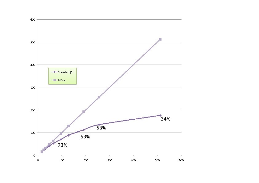
Beyond 300 computing cores, the sequential parts of the code start to dominate.
With more realistic computing parameters (ecut 40), they
dominate only beyond 600 processors.
This last example is the end of the present tutorial. You have been explained the
basics of the current implementation of the parallelism for the linear-response
part of ABINIT, then you have explored two test cases : one for a small cell materials,
with lots of k points, and another one, medium-size, in which the k point and band parallelism
can be used efficiently even for more than one hundred computing cores.